In this lecture, we continue to work on the complexification - combining two complex numbers via transforming one of them into either polar or Cartesian form. After getting the solution of input-output systme using complexification, we investigate some properties of the output as system and input parameters vary. The same framework will be applied to study the input-output system for the 2nd order ODEs. Lastly, we learn how to analyze autonomous ODEs without actually obtaining solutions. The stability of the fixed points plays the central role here.

Complexification II

In the last lecture, we learned that the real or imaginary part (depending on the forcing function) of the solution of a complexfied ODE becomes the solution of the original problem. Consider the following complexified ODE

\begin{equation} \hat T’ + k \hat T = k e ^{ i \omega t } \end{equation}

and its steady-state solution

\begin{equation}\label{eq:cx_solution}\tag{1} \hat T = \frac{ 1 }{ 1 + i ( \frac{ \omega }{ k } ) } e ^{ i \omega t }. \end{equation}

Note that it is given in an awkward form because the Cartesian and polar forms are mixed together. To take the real part, we need to transform one of them into the other form. First, we represent \eqref{eq:cx_solution} in polar form and take the real part. A complex number $z$ can be written in polar form as

$z = x + i y = r e ^{ i \theta },$

where $r = \sqrt{ x ^2 + y ^2 } $ and $\theta = \tan ^{-1} { (\frac{ y }{ x }) } $ are called the modulus (magnitude) and the argument (phase), respectively. Thus, the denominator of the first part of \eqref{eq:cx_solution} can be written as $ \sqrt{ 1 + ( \frac{ \omega }{ k } ) ^2 } e ^{ i \phi } $ where $ \phi = \tan ^{-1} ({\frac{ \omega }{ k }}) $. From the following relationship between $z$ and $ 1/z $,

\begin{equation} z \frac{ 1 }{ z } = 1 = 1 e ^{ i \, 0 } \end{equation}

and the properties of multiplication in polar form,

\begin{equation} r _1 e ^{ i \theta _1 } r _2 e ^{ i \theta _2 } = r _1 r _2 e ^{ i ( \theta _1 + \theta _2 ) } \end{equation}

we observe that

\begin{equation} r _1 r _2 = 1 \Rightarrow r _2 = \frac{ 1 }{ r _1 } \quad \textrm{and} \quad \theta _1 + \theta _2 = 0 \Rightarrow \theta _2 = - \theta _1, \end{equation}

from which we obtain

\begin{equation} \frac{ 1 }{ 1 + i ( \frac{ \omega }{ k } ) } = \frac{ 1 }{ \sqrt{ 1 + ( \frac{ \omega }{ k } ) ^2 }} e ^{ - i \phi }. \end{equation}

Finally, the solution \eqref{eq:cx_solution} becomes

\begin{equation} \hat T = \frac{ 1 }{ \sqrt{ 1 + ( \frac{ \omega }{ k } ) ^2 }} e ^{ - i \phi } e ^{ i \omega t } = \frac{ 1 }{ \sqrt{ 1 + ( \frac{ \omega }{ k } ) ^2 }} e ^{ i ( \omega t - \phi) }. \end{equation}

and the solution of the original problem (with $ \cos { \omega t } $ forcing function) becomes the real part of the above equation

\begin{equation} T = \frac{ 1 }{ \sqrt{ 1 + ( \frac{ \omega }{ k } ) ^2 }} \cos { ( \omega t - \phi) }. \end{equation}

Next, we transform \eqref{eq:cx_solution} into Cartesian form. Using Euler’s formula, we get

$\begin{equation}\begin{aligned} \frac{ 1 }{ 1 + i ( \frac{ \omega }{ k } ) } e ^{ i \omega t } &= \frac{ 1 }{ 1 + i ( \frac{ \omega }{ k } ) } ( \cos \omega t + i \sin \omega t ) \\ &= \frac{ 1 - i ( \frac{ \omega }{ k } ) }{ 1 + ( \frac{ \omega }{ k } )^2 } ( \cos \omega t + i \sin \omega t ) \end{aligned}\end{equation}$

of which the real part is

$\begin{equation} \frac{ 1 }{ 1 + ( \frac{ \omega }{ k } )^2 } \left\{ \cos \omega t + \left( \frac{ \omega }{ k } \right) \sin \omega t \right\} \end{equation}$

The problem with the above formula is that we cannot get any meaningful interpretation. We need to rewrite it into physically meaningful way. Using the following formula

$\begin{equation} A cos \theta + B \sin \theta = \sqrt{ A ^2 + B ^2 } \cos ( \theta - \psi ), \quad \psi = \tan ^{ -1 } \left( \frac{ B }{ A } \right) \end{equation}$

we get

$\begin{equation} T = \frac{ 1 }{ 1 - ( \frac{ \omega }{ k } )^2 } \left\{ \sqrt{ 1 + (\frac{ \omega }{ k }) ^2 } \cos ( \omega t - \phi ) \right\} = \frac{ 1 }{ \sqrt{ 1 + ( \frac{ \omega }{ k } ) ^2 }} \cos { ( \omega t - \phi) }. \end{equation}$

Some characteristics of the response

Consider again the cooling equation

\begin{equation} T’ + k T = k \cos \omega t , \end{equation}

and note that there are two parameters $k$ and $\omega$ where the former is related with the system and the latter with the forcing. Now, we investigte how the change of these parameter values affect the response of the system. From the solution

\begin{equation} T = \frac{ 1 }{ \sqrt{ 1 + ( \frac{ \omega }{ k } ) ^2 }} \cos { ( \omega t - \phi) }, \quad \phi = \tan ^{-1} ({\frac{ \omega }{ k }}), \end{equation}

we observe that $ \frac{ 1 }{ \sqrt{ 1 + ( \frac{ \omega }{ k } ) ^2 }} $ represents the maximum amplitude of the response and $ \phi $ represents the phase lag. In the following figure, black and read lines are input and output (steady-state part), respectively. (Warning!) There is an error in the figure. Try to find it out.

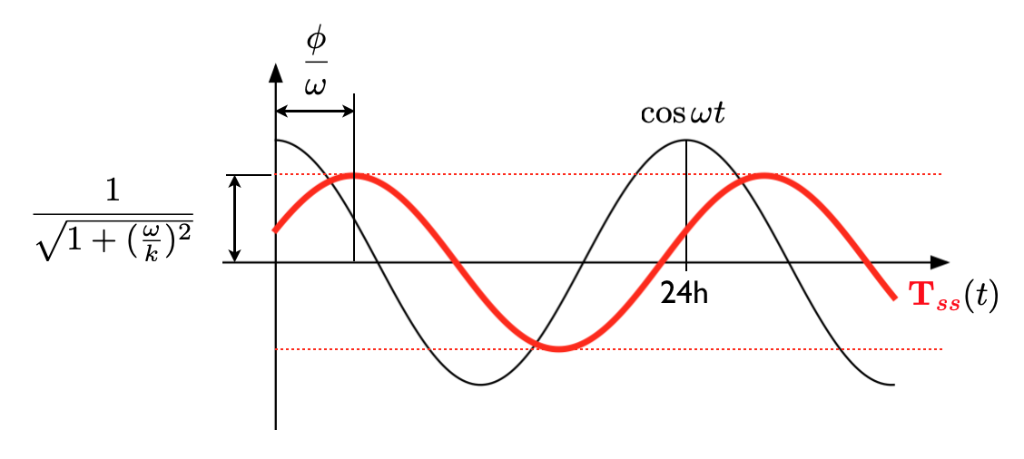
As $k$ increases we can see that the magnitude is getting bigger and the phase lag getting smaller. This is physically reasonable since high values of $k$ implies poor insulation. (Why?)

Autonomous ODEs

The first order autonomous ODEs are given in the following form,

\begin{equation}\label{eq:autonomous-1st}\tag{2} y’ = f(y). \end{equation}

Note that the RHS is a function of $y$ only which is different from the general form. Due to this fact, we can guess the behavior of the solution of \eqref{eq:autonomous-1st} without too much difficulties. One of the well-known first order autonomous ODEs is the logistic equation

\begin{equation} y’ = Ay - B y ^2. \end{equation}

This models the population growth and a modified version of Malthus theory. The first term in the RHS represents the exponential growth of population as Malthus predicted and the second term reflects the control due to the limitation of resources such as land and food. Note that the second term does not affect too much when the value of $y$ is relatively small but kicks in as $y$ increases. The starting point of the analysis of autonomous ODEs is to get the fixed points and their stability.

Stability of fixed points

The fixed points of autonomous ODEs are the values of $y$ which satisfy

\begin{equation} f(y) = 0. \end{equation}

Since the above equation implies that $y’ = 0$, if $y$ is at a fixed point, it does not move at all. This is why they are called fixed points or stationary or solutions or equilibrium (equilibria). After getting the fixed points, we need to check their stability. Stability of a fixed point is determined by the behavior of a solution as it is quite near to a fixed point. (More detailed and rigorous definition of the stability will be given later.) In this perspective, the concept of stability is locally defined - it does not say anything when the solution is far away from the fixed point. In the first order ODEs, we have three types of stabilty: stable, unstable, and semistable. (Again, more complex stability cases will be given later.)