In this lecture, we consider a 1st-order ODE as an input-output system. This type of ODE is given in a non-homogeneous form. As we have seen in the cooling example, the temperature of a house changes as the external temperature changes. Here, we consider the external temperature as an input and the temperature of the house as an output. This view is quite important because many of real world problems can be seen in this way and our interest is usually to find out the relationship between those two. Next, we learn how to solve non-homogeneous ODEs with sinusoidal forcing using complexification.

System response of 1st-order ODEs

We consider the cooling equation when the external temperature is also a function of time.

\begin{equation} \frac{ dT }{ dt } = k (T _e (t) - T) \end{equation}

When the exteranl temperature was a constant, the equation was separable. But now, it is linear and can be written as

\begin{equation} T’ + kT = k T _e (t) \end{equation}

As stated previously, we are interested in the relation between input (force) and output (response). Though there are many ways to look at this relation, our approach is to measure the response when a sinusoidal force is applied. The reason for applying sinusoidal forces to a system is that they are simple to generate and they can make any shape of function if combined appropriately. (This is the topic of Fourier series.)

The solution of the above equation can be given as follow, see Lecture 4

\begin{equation} T(t) = \underbrace{k \int_0 ^t e ^{ -k(t-s) } T_e (s) ds}{\textrm{steady-state solution}} - \underbrace{T(0)e ^{ -kt }} {\textrm{transient solution}} \end{equation}

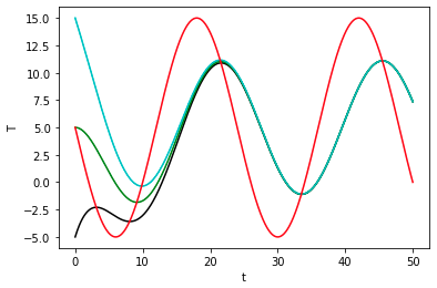
To observe how temperature of the house changes, we plot $ T(t) $ for different values of initial conditions.

## Define function
k = 0.2
def f(t, T):
	return k*(-10*np.sin(np.pi/12*t) + 5 - T)    

## Euler method & plot
t, T = forwardEuler(f,0,0.05,50,-5)
t1, T1 = forwardEuler(f,0,0.05,50,5)
t2, T2 = forwardEuler(f,0,0.05,50,15)

plt.figure()
plt.plot(t,T,'k')
plt.plot(t1,T1,'g')
plt.plot(t2,T2,'c')
plt.plot(t,T\_ext(t),'r')
plt.xlabel('t')
plt.ylabel('T')
plt.show()

One can easily see that the influence of transient solution disapears around $ t = 23 $. Next, we interpret the steady-state solution. Approximating the steady-state solution as summation, we have

$\begin{equation}\begin{aligned} T(t) &= k \int \_0 ^t e^{-k(t-s)} T\_e(s) ds \\ &\approx k \sum \_{i=1} ^N e^{-k(t-s\_i)} T\_e(s\_i) \Delta s\_i \end{aligned}\end{equation}$

where $ e ^{ -k(t-s_i)} T _e (s _i )$ represents the influence of the external temperature at $ t = s _i $ on the temperature of the house at current time $ t = t $. Thus, we can interpret the above equation as the current temperature of the house is the sum of all the influences starting from the initial time ( $ t = 0 $ ) to current time $t$.

Complexification I

Using complexification, we can easily solve non-homogeneous ODEs with sinusoical inputs. Consider

\begin{equation}\label{eq:linear_nonhomogeneous}\tag{1} T’ + kT = k \cos \omega t. \end{equation}

Instead of solving this directly, we solve the following complexified ODE,

\begin{equation} \hat{T}’ + k \hat{T} = k (\cos \omega t + i\sin \omega t ) = k e ^{ i\omega t } . \end{equation}

and take the real part of $ \hat{T} $ which becomes the solution of the original problem. The logic behind this is the linearity: if $x$ and $y$ are solutions of \eqref{eq:linear_nonhomogeneous}, their linearn combination $ cx + dy $ is also a solution. Let $ \hat{T} = T _r + i T _i $, where $ T _r $ and $ T _i $ are real and imaginary parts of $ \hat{T} $. By plugging this into the above equation, we have

$\begin{equation}\begin{aligned} (T _r + i T _i)' + k(T _r + i T _i) &= k (\cos \omega t + i \sin \omega t ), \\ T' _r + i T' _i + kT _r + i kT _i &= k\cos \omega t + i k \sin \omega t, \\ (T' _r + k T _r ) + i (T _i + k T _i ) &= k\cos \omega t + i k \sin \omega t. \end{aligned}\end{equation}$

Equating the real and imaginary parts on both sides, we obtain

\begin{equation} T’ _r + k T _r = k\cos \omega t, \quad \textrm{and} \quad T’ _i + k T _i = k \sin \omega t. \end{equation}