This is the second part of analytic solutions where we look into linear ODEs and Bernoulli equations. After studying how to solve these ODEs, we deal with existence and uniqness theorems. Refer to the following table to get a big picture.

	Basic Type	Variation
linear or nonlinear	Separable ODE	Homogeneous 1st-order ODE
linear or nonlinear	Exact ODE
linear	Linear ODE	Bernoulli Equation

Analytic Solutions II

First order linear ODEs

This group of ODEs is most popular in applications. Its general form is

\begin{equation} a(x) y’ + b(x) y = c(x) \end{equation}

We call this homogeneous if $ c(x)=0 $ and non-homogeneous otherwise i.e., $ c (x) \neq 0 $. Note that this is a linear equation: there is no nonlinear terms in $y$ or $y’ $ such as $ y^2 $ or $ {y’} ^ 3 $. Divide the above equation by $ a(x) $ and let $ p(x) = \frac{b(x) }{ a(x) } $, $ q(x) = \frac{ c(x) }{ a(x) } $, we get

\begin{equation}\label{eq:linear_st}\tag{1} y’ + p(x) y = q(x) \end{equation}

which is called a standard linear form. A solution of this ODE can be obtained by multiplying an integrating factor $ u(x) $,

\begin{equation} y’ u + p u y = q u \end{equation}

and make the LHS in the form of $ (yu)’ $. By comparing $ (yu)’ = y’u + yu’ $ with the LHS of the previous equation, we obtain $ yu’ = puy $ and thus

\begin{equation} u’ = pu \end{equation}

of which the solution is $ u = C e ^{ \int p(x) dx } $. Since we are multiplying this with every term of \eqref{eq:linear_st}, we can remove $C$ in the integrating factor. The procedure for solving linear ODEs is as follows:

Put it into a standard linear form
Calculate integrating factor, $u = e ^{ \int p(x) dx } $
Multiplying $u$ with every term in the ODE
Integrate

Example. Solve \begin{equation} \frac{ dT }{ dt } = k (T _e (t) - T) \end{equation}

Solution. First, note that this is not separable. (Why?) Putting it into a standard linear form,

\begin{equation} \frac{ dT }{ dt } + k T = k T _e (t) \end{equation}

Multiplying an integrating factor $ u = e ^{ \int k dt } = e ^{ kt } $, we get

\begin{equation} T’ e ^{ kt } + k T e ^{ kt } = k T _e (t) e ^{ kt } \end{equation}

Now integrate this, but use a definite integral instead of an indefinite one,

\begin{equation} \int _0 ^t \frac{ d }{ ds } (T e ^{ ks } ) ds = \int _0 ^t k T _e (s) e ^{ ks } ds. \end{equation}

After some manipulation, we obtain

\begin{equation} T(t) = k \int _0 ^t T _e (s) e ^{ -k(t - s) } ds + T(0) e ^{ - kt } \end{equation}

Note that the second term on the RHS goes to $0$ while the first term does not. We call the first term steady-state solution and the second one transient solution.

The last example can be considered as a model for an force-response (or input-output) relation. The solution represents how a system (e.g., temperature of a house) responses as an input (external temperature) varies. It is worth while to note that this is what most engineers need to know about a system of their interest.

Exercise. Solve $xy' + 2y = 4 x ^2$

Exercise. Solve \begin{equation} (1 + \cos x ) y’ - \sin {xy} = 2x \end{equation}

Bernoulli equation

The standart form of a Bernoulli equation is

\begin{equation} y’ + p(t) y = q(t) y ^\alpha.
\end{equation}

The above equation is nonlinear (why?) but can be tranformed into a first order linear ODE. We first divide the equation by $ y ^{ \alpha } $,

\begin{equation} y’ y ^{ -\alpha } + p(t) y ^{ 1 - \alpha } = q(t). \end{equation}

Using the substitution $ u = y ^{ 1 - \alpha } $ and its derivative $ u’ = (1 - \alpha ) y ^{ -\alpha } y’ $, we get

\begin{equation} \frac{ 1 }{ 1 - \alpha } u’ + p(t) u = q(t) \end{equation}

which is a first order linear ODE.

Exercise. Solve $y' = \epsilon y - \sigma y ^3 .$

The Existence & Uniqueness theorem

Before stating the theorems, we first ask why do we need to care about existence and uniqueness of solutions. So far we obtained solutions of many different ODEs analytically (existence) and by setting initial conditions, the solutions were uniquely determined (uniqueness). A problem comes in when we cannot solve ODEs. Consider the following IVP,

\begin{equation} y’ = x ^2 + y ^2, \quad y(0) = 1. \end{equation}

Since we cannot solve this ODE analytically, we try numerical methods to get the solution. But how do we know ‘the solution’ obtained numerically is actually a solution. It might have come from numerical errors and just looked like a solution. Of course, this does not happen for simple problems like the one given above. But when the equation is very complecated, we are not sure whether the numerically obtained solution could be a solution because there is no guarantee that even a solution exists. Thus, it is desirable to check whether a solution exists in the first place. However, mere existence does not tell us whether the given solution is unique, which leads us to the uniqueness problem.

Theorem. [Boyce & DiPrima 2.8] Consider the initial value problem (IVP) \begin{equation}\label{eq:uniqueness_standard_form}\tag{1} y’ = f(t,y), \quad y(0) = y _0 . \end{equation} If $f$ and $ \frac{ \partial f }{ \partial y } $ are continuous in a rectangle $ R: |t| \le a, \, |y| \le b $, then there is some interval $ |t| \le h \le a $ in which there exists a unique solution $ y = \phi (t) $ of the above initial value problem.

Proof. The proof is given here.

Example. Solve \begin{equation}\label{eq:uniqueness_example}\tag{2} xy’ = y - 1, \quad y(0) = 1. \end{equation}

Solution. Since this is a separable ODE, we have

$\begin{equation}\begin{aligned} \frac{ dy }{ y - 1 } &= \frac{ dx }{ x } \quad (x \neq 0) \\ \ln |y - 1 | &= \ln |x| + c \_1, \\ |y - 1 | &= cx. \\ \end{aligned}\end{equation}$

Thus, we have $ y = cx + 1, \, (x \neq 0) $. Considering the intial condition, there are infinite number of solutions emanating from $ (0,1) $. Note also that $ y \equiv 1 $ is also a solution. A few solutions are shown in the following figure.

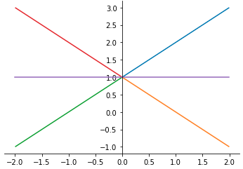
Note that there are infinite number of solutions at $ x = 0, y = 1 $ and no solution along the $y$-axis except $ y = 1 $. Putting \eqref{eq:uniqueness_example} into the form of \eqref{eq:uniqueness_standard_form}, we have $ f(t,y) = \frac{ y - 1 }{ x } $ and $ \frac{ \partial f }{ \partial y } = \frac{ 1 }{ x } $ both of which are not continuous near $ (0, 1) $, thus existence and uniqueness are not guaranteed near that point.

Example. Solve \begin{equation}\label{eq:uniqueness_example2}\tag{3} y’ = 3t y ^{ 1/3 } , \quad y(0) = 0. \end{equation}

Solution. This is also separable, we get

$\begin{equation}\begin{aligned} \frac{ dy }{ y ^{ 1/3 } } &= 3t \\ y ^{ 2/3 } &= t ^2 + c. \end{aligned}\end{equation}$

The solution becomes $ y = ( t ^2 + c) ^{ 3/2 } $. The initial condition is satisfied if $ c = 0 $, so $ y = ( t ^2 ) ^{ 3/2 } $. Since $ y \equiv 0 $ is also a solution, the uniqueness is violated at $ (0, 0) $.

Exercise. Check the conditions for existence and uniqueness for the above problem.

References

Haynes Miller, and Arthur Mattuck. 18.03 Differential Equations. Spring 2010. Massachusetts Institute of Technology: MIT OpenCourseWare, https://ocw.mit.edu.
William Boyce, and Richard DiPrima, Elementary Differential Equations, John Wiley & Sons, 7th edition, 2001