Analytic solutions mean that solutions can be written in terms of elementary functions such as polynomials, trigonometric function, exponential functions, and hyperbolic functions. There are a few types of first-order ODEs which we can solve analytically. These types are separable, exact, and linear. In the subsequent lectures, we will deal with each of them. It is worth while to note that in the first two cases, the ODE could be nonlinear while in the last case, it should be linear as the name implies. In this world of the first-order ODEs, we will meet the first and the third ones most frequently. We will also meet a few peculiar looking ODEs that don’t look like one of these types at first sight but actually could be reduced to these cases by a certain transformation. (See the following table.)

	Basic Type	Variation
linear or nonlinear	Separable ODE	Homogeneous 1st-order ODE
linear or nonlinear	Exact ODE
linear	Linear ODE	Bernoulli Equation

Analytic Solutions I

Separable ODEs

The first ethnic group of this ODE world is called separable. The reason for this name will be clear soon. The specialty of this group is that the function in the right-hand side (RHS) of the general form is separated into a multiple of two functions each of which has a different variable $x$ and $y$, i.e., $ f(x,y) = g(x)/h(y)$ . Thus

\begin{equation}\label{eq:sep_ode}\tag{1} \frac{dy}{dx} = \frac{ g(x)}{ h(y) }, \end{equation}

and by a simple manipulation, we obtain

\begin{equation}\label{eq:dseparable}\tag{2} h(y) dy = g(x) dx. \end{equation}

Clearly, LHS and RHS are functions of a different variable, thus the original ODE is separated. Now we can integrate each side separately with respect to $y$ and $x$,

\begin{equation} \int h(y) dy = \int g(x) dx + C \quad \textrm{or} \quad H(y) - G(x) = C, \end{equation}

which gives us a solution to \eqref{eq:sep_ode}. Note that the $ H(x) $ and $ G(x) $ are antiderivatives of $ f(x) $ and $ g(x) $. One might wonder how we could integrate \eqref{eq:dseparable} separately for $x$ and $y$ to obtain a solution. To see this, let us consider

\begin{equation} h(y) \frac{dy }{ dx } = g(x) \quad \textrm{or} \quad h(y) \frac{dy }{ dx } - g(x) = 0. \end{equation}

Integrating with respect to $x$, we get

$\begin{equation}\begin{aligned} \int \left\{ h(y) \frac{dy }{ dx } - g(x) \right\} dx &= \int h(y) \frac{dy }{ dx } dx - \int g(x) dx \\ &= \int \frac{ dH }{ dy } \frac{dy }{ dx } dx - \int g(x) dx \\ &= \int \frac{ dH }{ dx } dx - \int g(x) dx \\ &= H(y) - G(x) = C, \end{aligned}\end{equation}$

where the third equality comes from chain rule.

Example 3.1 [Kreyszig 1.3] Solve $ y’ = -2xy $.

Solution. Notice that this is separable and can be written as

$\frac{ dy }{ y } = - 2 x \, dx$

Integrating both sides, we get

$\ln |y| = -x ^2 + C \_1.$

Exponentiating both sides gives us

\begin{equation}\label{eq:normal_ode_solution}\tag{3} |y| = C_2 e ^{-x ^2 } \quad \textrm{if } y \neq 0, \end{equation}

where $C_2 = e ^{ C _1 }$. Notice that $ y = 0 $ is also a solution. Here, we could write the solution as

\begin{equation}\label{eq:normal_ode_solution_no_abs}\tag{4} y = C e ^{-x ^2 } \end{equation}

because the constant $C$ takes care of the sign; if $ y > 0 $, we get \eqref{eq:normal_ode_solution_no_abs} by $ C = C _2 $ and if $ y < 0 $, \eqref{eq:normal_ode_solution} becomes $ -y = C_2 e ^{-x ^2 } $ which can be written in the form of \eqref{eq:normal_ode_solution_no_abs} by letting $ -C_2 = C $. Thus, the solution becomes

$\begin{equation} y = \left\{ \begin{array}{cl} C e ^{-x ^2 } & \textrm{if } y \neq 0 \\ 0 & \textrm{if } y = 0 \end{array} \right. \end{equation}$

Example 3.2 [Boyce & DiPrima 2.2] Solve the initial value problem (IVP)

\begin{equation}\label{eq:ivp_ode}\tag{5} \frac{dy}{dx} = \frac{ 3 x ^2 + 4 x + 2 }{ 2 (y - 1) }, \quad y(0) = -1. \end{equation}

Solution. Since this is separable, we have

\begin{equation} 2(y - 1) dy = (3 x ^2 + 4 x + 2 ) dx \end{equation}

Integrating both sides,

\begin{equation}\label{eq:ivp_gen}\tag{6} y ^2 - 2y = x ^3 + 2 x ^2 + 2 x + C. \end{equation}

From the initial condition, we can find that $ C = 3 $ and the solution to the IVP is

\begin{equation}\label{eq:ivp_sol}\tag{7} y ^2 - 2y = x ^3 + 2 x ^2 + 2 x + 3. \end{equation}

Note that \eqref{eq:ivp_gen} is one of many (infinite) solutions to the given ODE while \eqref{eq:ivp_sol} is the solution which satisfies the initial value. Note also that the solution \eqref{eq:ivp_sol} is given in an implicit form. The explicit solution would be obtained by adding $1$ to both sides,

$\begin{equation}\begin{aligned} y ^2 - 2y + 1&= x ^3 + 2 x ^2 + 2 x + 4, \\ (y-1) ^2 &= x ^3 + 2 x ^2 + 2 x + 4, \end{aligned}\end{equation}$

which gives

\begin{equation}\label{eq:ivp_ex_sol}\tag{8} y = 1 \pm \sqrt{x ^3 + 2 x ^2 + 2 x + 4 }. \end{equation}

The last equation has two branches: one with positive and the other with negative sign. Thus, which one is the correct answer? (You can check this using the initial condition.) Finally, note that a solution of ODEs is not usually valid for all the values of $x$. In this example, the value in the square root should not be negative and from \eqref{eq:ivp_ode}, one can see that $ y = 1 $ cannot be a solution. Note that a solution of ODEs should be differentiable; in this example, $y$ is not differentiable at $ y = 1 $ since its derivative does not exist. Since the quantity in the square root can be factored into $ (x + 2) (x ^2 + 2) $, the solution \eqref{eq:ivp_ex_sol} is valid when $ x \in (-2, \infty) $. You can easily see these features from the following figure. (Blue line is the solution of IVP \eqref{eq:ivp_ode}.)

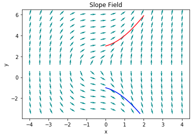
The following is the python code to draw the slope field shown above. Note that you also need to have forwardEuler code to run this.

x, y = np.mgrid[-4:4:16j, -3:6:16j] # create a grid on tx-plane
U = 1                               # calcuate a slope
V = (3*x**2 + 4*x + 2)/(2\*(y-1))

speed = np.sqrt(U**2 + V**2)        # calculate the size of a slope
UN = U/speed                        # normalize the size of a slope
VN = V/speed

plt.figure()  
plt.quiver(x, y, UN, VN,            # plot slopes at grid points
	       color='Teal', 
	       headlength=7)
plt.title('Slope Field')
plt.xlabel('x')
plt.ylabel('y')

# Euler method
def f1(x,y):
	return (3*x**2 + 4*x + 2)/(2*(y-1))
x1, y1 = forwardEuler(f1,0,0.0001,1.8,-1)
x2, y2 = forwardEuler(f1,0,0.0001,2,3)

# plot integral curve
plt.plot(x1,y1,'b')
plt.plot(x2,y2,'r')
plt.show()

Example 3.3 From the cone drop experiment in class, we found that a drag force can be written as $ F _d = c \rho A v ^2 $, where $c$ needs to be determined from experiment. From this and the Newton’s second law, a falling object can be modeled as $-mg + c \rho A v ^2 = m v'.$ Find its solution.

Solution. For simplicity, let $ k = c \rho A $, then the above equation becomes $ -mg + k v ^2 = m v’$. This ODE is separable because

$\begin{equation} \frac{ dv }{ dt } = -g + \frac{ k }{ m } v ^2 = \frac{ k }{ m } ( v ^2 - \frac{ m g }{ k } ), \\ \frac{ dv }{ v ^2 - a ^2 } = \frac{ k }{ m } dt \end{equation}$

where $ a = \sqrt{ \frac{ m g }{ k } } $. The next step will be given as an exercise.

Homogeneous first-order ODEs

In class, we call this as a variation of basic types because this can be transformed into the basic type by a simple change of variables. The homogeneous first-order ODEs are the ones that can be changed into the form of \begin{equation} y’ = F\left( \frac{ y }{ x } \right). \end{equation} For example,

$\begin{eqnarray} y' &= \frac{ x ^2 y }{ x ^3 + y ^3 } \Rightarrow y' = \frac{ \frac{ y }{ x } }{ 1 + \left(\frac{ y }{ x } \right) ^3 } \\ xy' &= \sqrt{ x ^2 + y ^2 } \Rightarrow y' = \sqrt{ 1 + \left(\frac{ y }{ x } \right) ^2 } \end{eqnarray}$

Then a change of variable: $ u = \frac{ y }{ x } $ transforms the above equations into the form of $ u + x u’ = F(u) $ which is separable. (Here, we use the fact that $ y = ux $ and $ y’ = u + x u’ $.)

This is how we solve the homogeneous first-order ODEs but how to check a given ODE can be transformed into this form. A simple check is to change $x$ and $y$ to $ cx $ and $ cy $. If the changed ODE have the same form as the original one, then it is a homogeneous first-order ODE.

Exact ODEs

Consider an equation \begin{equation}\label{eq:exact}\tag{9} \psi (x,y(x)) = C, \end{equation} and its differentiation with respect to $x$, \begin{equation}\label{eq:exact_ode}\tag{10} \frac{ d\psi }{ dx } = \frac{ \partial \psi }{ \partial x } + \frac{ \partial \psi }{ \partial y } \frac{ dy }{ dx } = 0. \end{equation} If an ODE is given in the following form \begin{equation}\label{eq:exact_variation}\tag{11} P(x,y) + Q(x,y) \frac{ dy }{ dx } = 0 \end{equation} or in its variations

$\begin{equation} P(x,y) dx + Q(x,y) dy = 0 \\ \frac{ dy }{ dx } = - \frac{ P(x,y) }{ Q(x,y) } \end{equation}$

by comparing these with \eqref{eq:exact_ode}, we can deduce that the solution to the given ODE is actually \eqref{eq:exact} if $ P(x,y) = \frac{ \partial \psi }{ \partial x } $ and $ Q(x,y) = \frac{ \partial \psi }{ \partial y } $. Note that $ \psi(x,y(x)) = C $ defines $ y(x) $ implicitly. If this is the case, we call these ODEs exact. Before getting further, consider the following example.

Example 3.4 Solve the following ODE.
$(y \cos x + 2 x e ^y ) + ( \sin x + x ^2 e ^y - 1) y' = 0.$

Solution. It is easy to see that the above equation is given in the first form. To solve this, we first need to check that this is indeed equivalent to \eqref{eq:exact_ode}. Then, we find a function $ \psi(x,y(x)) = C $ which satisfies the equation. To check the first step, we use a fact from multivariable calculus: the order of differentiation doesn’t matter (This is true if a function is smooth enough.), e.g. $ \frac{ \partial^2 \psi }{ \partial x \partial y } = \frac{ \partial^2 \psi }{ \partial y \partial x }$. Thus, if $ P(x,y) = \frac{ \partial \psi }{ \partial x } $ and $ Q(x,y) = \frac{ \partial \psi }{ \partial y } $ then the following criteria should be satisfied.

\begin{equation}\label{eq:exact_check}\tag{12} \frac{ \partial P }{ \partial y } = \frac{ \partial Q }{ \partial x}. \end{equation}

Since $ P(x,y) = y \cos x + 2 x e ^y $ and $ Q(x,y) = \sin x + x ^2 e ^y - 1 $, $ \frac{ \partial P }{ \partial y } = \cos x + 2 x e ^y = \frac{ \partial Q }{ \partial x }$. The next step would be finding a solution $\psi$ in the following way. First, integrate $ P $ with respect to $x$ or $ Q $ to $y$. Then $ \psi(x,y) = \int P(x,y) dx = y \sin x + x ^2 e ^y + C_1(y) $, $ \frac{ \partial \psi }{ \partial y } = \sin x + x ^2 e ^y + C_1’(y) $. By comparison, $ C_1’(y) = -1 $ and $ C_1(y) = -y + C _2 $. Thus $ \psi(x,y) = y \sin x + x ^2 e ^y - y = C $. Even though we get a solution, this is not always guaranteed. This is because the criteria \eqref{eq:exact_check} is actually necessary condition for exactness. I.e., if \eqref{eq:exact_variation} is exact, then \eqref{eq:exact_check} holds but not the converse. To see this, consider the following ODE,

$\frac{ -y }{ x ^2 + y ^2 } dx + \frac{ x }{ x ^2 + y ^2 } dy = 0.$

Note that the exactness critria \eqref{eq:exact_check} is satisfied for this equation, where $ P(x,y) = \frac{ -y }{ x ^2 + y ^2 } $ and $ Q(x,y) = \frac{ x }{ x ^2 + y ^2 } dy $. However, we cannot find the function $\psi$ which satisfies $ P = \frac{ \partial \psi }{ \partial x } $ and $ Q = \frac{ \partial \psi }{ \partial y } $. This is because the domain of this problem is not simply connected, i.e., the above ODE is defined in $ \mathbb{R} ^2 - \left\{ (0,0) \right\} $. However, with some additional conditions, \eqref{eq:exact_check} becomes a necessary and sufficient condition as shown in the next theorem.

Theorem. A necessary and sufficient condition for $P(x,y) + Q(x,y) \frac{ dy }{ dx } = 0$ to be exact is $\frac{ \partial P }{ \partial y } = \frac{ \partial Q }{ \partial x}$ where $P$ and $Q$ and their partial derivatives are continuous in a domain of our interest, which is simply connected.

By checking that $P$ and $Q$ satisfy the above theorem and the domain is simply connected, one can check the exactness of ODE just from \eqref{eq:exact_check}.

Supplement

To understand the physical meaning of exact ODEs, it is unavoidable to deal with some of the core concepts of vector calculus. Here, we briefly and briskly review those concepts that are needed to understand exact ODEs. A conservative vector field is a vector field $ \mathbf{F} $ obtained from the gradient of a scalar function (potential function) $ \psi( x,y,z ) $ such that

\begin{equation}\label{eq:gradient}\tag{1} \mathbf{F} = \nabla \psi, \end{equation}

where $ \nabla $ is a del operator and defined as $\nabla = \frac{\partial }{\partial x} \mathbf{i} + \frac{\partial }{\partial y} \mathbf{j} + \frac{\partial }{\partial z} \mathbf{k}$ in Cartesian coordinates. Thus we have

\begin{equation}\label{eq:vector_field}\tag{2} \mathbf{F} = \frac{\partial \psi }{\partial x} \mathbf{i} + \frac{\partial \psi }{\partial y} \mathbf{j} + \frac{\partial \psi }{\partial z} \mathbf{k} = \left( \frac{\partial \psi }{\partial x}, \frac{\partial \psi }{\partial y}, \frac{\partial \psi }{\partial z} \right) = (F _1, F _2, F _3 ). \end{equation}

We can show that an integration in a conservative vector field is path independent

$\int _{C\_1} \mathbf{F} \cdot \hat{\mathbf{t}} \, ds = \int _{C\_2} \mathbf{F} \cdot \hat{\mathbf{t}} \, ds,$

or equivalently,

\begin{equation}\label{eq:zero_circulation}\tag{3} \oint _C \mathbf{F} \cdot \hat{\mathbf{t}} \, ds = 0, \end{equation}

since

$\int _C \mathbf{F} \cdot \hat{\mathbf{t}} \, ds = \int _C \frac{ d \psi }{ ds } ds = \psi (x _2, y _2, z _2 ) - \psi (x _1, y _2, z _2 ),$

which implies the path independence. (If an integration over a path $C$ depends only on the end points, it is path independent and becomes zero when evaluated over a closed curve.) The first equality in the above equation comes from the following inner product,

$\mathbf{F} \cdot \hat{\mathbf{t}} = \frac{\partial \psi }{\partial x} \frac{ dx }{ ds } + \frac{\partial \psi }{\partial y} \frac{ dy }{ ds } + \frac{\partial \psi }{\partial z} \frac{ dz }{ ds } = \frac{ d \psi }{ ds },$

where, $\hat{\mathbf{t}} = \left( \frac{ dx }{ ds }, \frac{ dy }{ ds }, \frac{ dz }{ ds } \right) $ is a unit tangent vector along the curve $C$. From the definition of curl $\mathbf{F} = \nabla \times \mathbf{F}$

\begin{equation} \mathbf{n} \cdot \nabla \times \mathbf{F} := \lim_{\Delta S \to 0} \frac{ 1 }{ \Delta S } \oint _{ C} \mathbf{F} \cdot \hat{\mathbf{t}} \, ds \end{equation}

and zero circulation \eqref{eq:zero_circulation}, we have curl $ \mathbf{F} = 0 $. (If \eqref{eq:zero_circulation} holds, we get $ \mathbf{n} \cdot \nabla \times \mathbf{F} = 0$. Since the closed curve $C$ can be chosen arbitrarily, so is the direction of the unit normal vector $ \mathbf{n} $, which gives us the desired result.) In Cartesian coordinates, curl $ \mathbf{F} = 0 $ can be written as

\begin{equation} \left( \frac{\partial F _2}{\partial z} - \frac{\partial F _3}{\partial y} \right) \mathbf{i} + \left( \frac{\partial F _1}{\partial x} - \frac{\partial F _3}{\partial z} \right) \mathbf{j} + \left( \frac{\partial F _1}{\partial y} - \frac{\partial F _2}{\partial x} \right) \mathbf{k} = 0, \end{equation}

which implies \begin{equation}\label{eq:curl_free_check}\tag{4} \frac{\partial F _2}{\partial z} = \frac{\partial F _3}{\partial y}, \quad \frac{\partial F _1}{\partial x} = \frac{\partial F _3}{\partial z}, \quad \frac{\partial F _1}{\partial y} = \frac{\partial F _2}{\partial x}, \end{equation}

which are exactness criteria. Thus, we have shown that

$\mathbf{F} = \nabla \psi \Rightarrow \oint\_C \mathbf{F} \cdot \hat{\mathbf{t}} \, ds = 0 \Rightarrow \textrm{curl} \, \mathbf{F} = 0.$

How about the converse? That is, if $ \textrm{curl} \, \mathbf{F} = 0 $ then $ \mathbf{F} $ is a conservative vector field? The answer is - not always. The converse is valid only if the conditions given in the above theorem are satisfied. If so, then the condition \eqref{eq:exact_check} tells us whether an ODE comes from a conservative vector field.