In the previous class, we looked at a cooling problem. Using a physical principle, we could model this problem as a differential equation which is classified as the first order ordinary differential equations (ODEs). In the first part of this course, we will investigate various types of the first order ODEs and their solution methods.

A general form of the first-order ODEs.

A general form of the first-order ODEs can be written as

\begin{equation} \label{eq:1ode}\tag{1} y’ := \frac{dy}{dt} = f(t,y) \end{equation}

where $f$ is a function of two variables $t$ and $y$. It is called first-order because the highest derivative shown in the above equation is 1st-order, not higher orders like $ y’’ $ or $ y’’’ $. (We will deal with higher-order ODEs in the later part of this course.) The term ordinary differential means that $y’$ is a function of one variable only, in this case time $t$; if we consider changes of $y$ at many different places in addition to time, we would use $y(t,x)$ instead of $ y(t) $ and the rate of change of $y$ with respect to $t$ is written as $ \frac{ \partial y }{ \partial t } $. The equations with this type of derivative are called partial differential equations (PDEs). We will study PDEs in the next semester.

Other terms of interest are independent and dependent variables. Since we are interested in how $y$ changes as $t$ changes, $y$ is called a dependent variable while $t$ is called an independent one. Depending on authors or problems, many different symbols are used for independent and dependent variables. We have been using $t$ as an independent variable because the dependent variable $y$ changes in time. If it varies over a space, we had better use $x$ instead of $t$. In this case, the general form can be written as $ y’ = f(x,y) $. To make you confuse further, we may write the same differential equation as $ x’ = f(t,x) $. (Guess what is the dependent variable.)

The cooling equation, we considered in Lecture 1, is given as

\begin{equation} T’ = k(T_e - T), \end{equation}

where the right hand side is a function of a dependent variable $T$ only because $ T_e $ is assumed to be a constant. In this case, the general form can be given as $ y’ = f(y) $ which is called an autonomous equation. If we consider a variation of the external temperature, for example $ T_e(t) = k \sin t $, then the cooling equation becomes $ T’ = k(\sin t -T )$ and the right hand side is a function of $t$ and $T$, which is in the same form as \eqref{eq:1ode}.

Approximte Solutions.

Regardless of the simple look of the first order ODEs \eqref{eq:1ode}, they don’t usually yield analytic solutions. Here, analytic means that the solution is given in terms of elementary functions such as polynomials, trigonometric functions, exponential functions, and hyperbolic functions. (Hereafter, we will use analytic and closed form solutions interchangeably.) As we have seen in class, $ y’ = t/y $ and $ y’ = y -t ^2 $ are solvable while $ y’ = t - y ^2 $ is not. There are two questions that naturally arise here:

Q1. How do we know whether the given ODE is analytically solvable or not?
Q2. What can we do with it if it is not solvable?

In Lecture 3 and forward, we will answer to the first question by studying specific forms of the first-order ODEs that can be solved in closed forms. We deal with the second question in this lecture. Our approach is twofold: geometric and numerical.

Geometric view of ODEs: Drawing a slope field

For the cooling problem, we derived the following first-order ODE

\begin{equation}\tag{2} \frac{dT(t)}{dt} = k(T_e - T(t)). \end{equation}

To see how the solution of this equation behaves, we use $ t-T $ plane and draw some solutions on it. Let $ T_e = 5$ and $k = 0.1$. Since the left-hand side of the above equation (LHS) is a rate of change of temperature at a certain time t, it can be represented by a slope. The value of the slope is determined by the RHS by setting a specific number to T(t). We can pick as many points as we want and draw corresponding slopes at those points. Let a computer do this tedious job for us.

%matplotlib inline
import matplotlib.pyplot as plt
import numpy as np

### set parameters
Te = 5
k = 0.1

### calculate slopes
t, T = np.mgrid[0:50:2.5, 0:25:2.5] # create a grid on tT-plane
U = 1                               
V = k * (Te - T)                    # RHS of the ODE

speed = np.sqrt(U**2 + V**2)        # calculate the size of a slope
UN = U/speed                        # normalize the size of a slope
VN = V/speed

### plot
plt.figure()                
plt.quiver(t, T, UN, VN,            # plot slopes at grid points
           color='Teal', 
           headlength=7)

plt.title('Slope field')
plt.xlabel('time')
plt.ylabel('Temperature')
plt.show()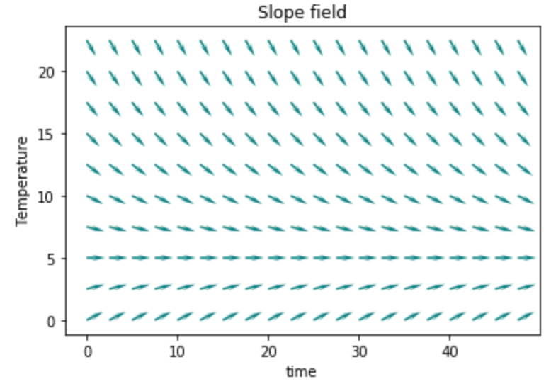

The above figure is called a slope (or direction) field since there are lots of slopes in the plane. You can draw some solutions of the ODE (2) on this slope field. Since any solution of (2) should satisfy the relation given in (2) for all $t$, it is a continuous smooth curve (why?) and its slope at any time $t$ should be tangent to the slope given in the slope field(why?). This curve is called an integral or solution curve.

There are a few points to ponder here: Firstly, What does $ T(0) $ represent? Since this is the value of the temperature at time $t = 0$, it is the temperature when you left the house. In mathematics, it is called an initial condition (IC) and the differential equation with IC

\begin{equation} \frac{dT(t)}{dt} = k(T_e - T(t)), \quad T(0) = C_0 \end{equation}

is called an initial value problem (IVP). Note that we can draw many integral curves in the slope field of an ODE, only one of them can be the solution of the IVP. Secondly, what do points on the $ T = 5 $ line represent? Is this line physically reasonable? If you started from any point on this line, you wouldn’t move up or down at all forever. This is called an equilibrium solution or a fixed point and is very important in the study of ODEs. We will delve into this later in this course. Lastly, do these integral curves remind you of any function you are familiar with? I hope it is not too hard to recognize that these curves look like $ e^{-t} $.

Geometric approaches are usually applied to the problems which cannot be solved analytically. By drawing a slope field with some integral curves, we could grasp a feeling of how the solution of the ODE behaves. However, even in the cases where closed form solutions could be obtained, geometric approaches help us interpret ODEs much better than closed form solutions as the following example demonstrates.

Exercise 2.1 Consider $ y’ = \sin { y } $ of which the solution is
$t = -\ln |\csc y + \cot y | + C.$
Can you see how the solution looks like? Even though one can get an exact solution, it is sometimes hard to interprete it. By drawing a slope field, you can easily see the behavior of the solution. Try to find it out.

To sum up, we can state what we have done as theorems.

Theorem 2.1 The integral curves are the graphs of the solutions to $ y’ = f(t,y) $.

Theorem 2.2 (Integral Curve Theorem)

Two integral curves cannot cross at an angle.

Two integral curves cannot be tangent to each other.

The above two statements can be given as an intersection priciple: Integral curves of $y’ = f(t,y) $ cannot intersect wherever $f(t,y)$ is smooth. A more detailed explanation is given here.

Exercies 2.2 Draw the slope field of the following equation. First on a piece of paper using isoclines and then using a computer.
$y' = x^2 + y^2 -1$

Numerical Approach: Euler’s Method

Euler’s method is the simplest numerical scheme that solves IVP. Even though it is impractical because of the problematic error handling, it is the basis of many high-order numerical schemes. We start with Euler’s method and delve into other schemes if time allows.

Consider the following IVP,

$\begin{equation}\begin{aligned} y'(t) &= f(t,y) \\ y(t_0) &= y_0 \end{aligned}\end{equation}$

If we discretize time with time step $h$, in other words, the value of $y$ at $t \in \{ 0, h, 2h, \ldots, T=nh \}$ instead of $ \{ t: 0 \le t \le T \} $, we have $ y’(t _n ) = f(t _n, y (t _n )) $. From calculus, we know that \begin{equation} y’(t_n) \approx \frac{y(t_n + h) - y(t_n)}{h}. \end{equation} Thus, we get \begin{equation} f(t _n, y (t _n )) \approx \frac{y(t_n + h) - y(t_n)}{h}, \end{equation} from which we obtain \begin{equation} y(t _n + h) \approx y(t _n ) + h f(t _n , y (t _n )) \end{equation} Let $ t _{ n + 1 } := t _n + h $ and $ y _n \approx y(t _n ) $, we have Euler’s method, \begin{equation} y _{ n + 1 } = y _n + h f (t _n , y _n ). \end{equation}

Now, we have a python code for Euler’s method.

def forwardEuler(f,t0,dt,tf,y0):
    """ forwardEuler uses the Euler algorithm to solve 
        the following initial value problem (IVP)
            
            y' = f(t, y)      ODE
            y(t0) = y0        IC
    
    f is the fuction on the right-hand side of the ODE
    t0 is the starting time
    dt is the timestep
    tf is the ending time
    y0 is the initial state of y
    
    This routine returns a tuple of the form (t, y)
    where t is a list of all of the times from t0 to tf
    in steps of dt """
    t = []
    y = []
    t.append(t0)
    y.append(y0)
    n = int((tf - t0)/dt) 
    
    for i in range(n):
        ytemp = y[i] + f(t[i],y[i])*dt
        ttemp = t[i] + dt

        y.append(ytemp)
        t.append(ttemp)
    return np.array(t), np.array(y)

Example 2.1 Solve the following IVP using Euler method.
$\frac{dy}{dt} = y + t, \quad y(0) = 0.$

Solution: We first define a function

### define a function
def f(t,y):
    return y + t

and call Euler’s method.

### define a function
t, y = forwardEuler(f,0,0.2,1,0)

plt.figure()
plt.plot(t,y)
plt.xlabel('t')
plt.ylabel('y')
plt.show()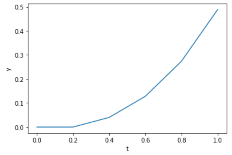

Exercise 2.3 Solve the following IVP using Euler method.
$y' = 1 + t - y, \quad y(1) = 3.$

Exercise 2.4 Draw a slope field of the following ODE and draw some integral curves on the slope field.
$y' = 1 + t - y.$

Exercise 2.5 Draw a slope field of the following ODE and draw some integral curves on the slope field.
$t\frac{dy}{dt} + 2y = 4t^2.$

After finding out how versatile the numerical method is, you may ask: Why not use computers in the first place? What is the use of the geometric approach or analytical methods that we are going to study? A short answer would be that you may end up with a result that could be catastrophic if the numerical method is used blindly. There are many pitfalls in numerical methods such as

Some problems are quite subtle that small errors add up producing quite different results. link

Before applying numerical schemes, it is always a good idea to get a ballpark measure by solving similar but simpler problem using analytical or geometric methods.

References

Haynes Miller, and Arthur Mattuck. 18.03 Differential Equations. Spring 2010. Massachusetts Institute of Technology: MIT OpenCourseWare, https://ocw.mit.edu.
Steven H. Strogatz, Nonlinear Dynamics And Chaos: With Applications To Physics, Biology, Chemistry, And Engineering, Westview Press, 2nd edition, 2015